Tag: Data Preparation

  • The Post that Started it All: What is Business Intelligence?

    Concepts covered in this article: Business Intelligence, Four Broad Disciplines


    Whenever I answer the question “what do you do for work?”, the next question I typically get is “what’s business intelligence?” Since those two questions are the very same ones that started me on my journey in this field, I thought it’d be an appropriate place to start this series of articles. 

    Business intelligence is about having the right information at the right time in order to make informed decisions for your business. The form this information takes can vary widely – ranging from a piece of paper you carry in your pocket, to bank statements, all the way to a set of digital reports that update automatically and answer all sorts of questions. Business intelligence (or, as I’ll refer to it often here, ‘BI’) doesn’t have to apply just to business either; the same tools used by retailers and manufacturers can be used to support public health decisions, research projects, nonprofit causes, or personal goals. 

    The above definition is what the users experience, and what we at Source to Share work to provide. However, there’s a whole world going on underneath the final reports that the user doesn’t see. That world can be separated into 4 broad disciplines that progress naturally from one to the next. 

    Four Broad Disciplines of Business Intelligence 

    1. Data Prep 
      This is usually the first step in any sort of BI process. Data prep usually starts with literally finding the data (it isn’t always in one place), then looking at it to make sure it’s valid. To prepare the data for modeling, oftentimes it will be changed from one format to another, and tables will be combined, split apart, and/or cleaned up. Then the whole slew will be loaded into reporting software. 
    1. Data Modeling 
      This is the practice of organizing data into meaningful groupings (customers, products, sales, etc.) and defining relationships between them. The modeling we engage in is called ‘semantic modeling’, and it enables users to easily locate data (or attributes) and navigate their relationships. 
    1. Data Measurement 
      This is the practice of overlaying computations on the dataset. This could be as simple as summing up sales so we can know just how many widgets we’ve sold (and comparing that to our widget budget), or as complicated as forecasting how many widgets we expect to sell next spring. 
    1. Data Visualization 
      This is an often-overlooked discipline in BI, but VERY important. Not all visualizations are equally useful, and some, like the common pie chart, are as overused as they are ineffective at conveying information accurately. The reports created in this step are what’s used to drive decision-making, and there is both a science and an art to creating useful, beautiful reports. 

    It’s important to note that during a BI project, we’ll often jump around from one discipline to the next. After some basic data prep and data modelling, we might start mocking up some crude visualizations. As we run into challenges creating reports, we’ll work to solve them at whatever stage is best. Often it is much more effective to solve problems upstream, which is the topic of an entire article later in this series. 

    I created this article and the rest of the series as I tried to answer the question ‘what is Business Intelligence?’ in greater and greater depth. They’re designed as a learning tool for myself and others – a way to document my learning and create a space for the rest of the crew at Source to Share to give feedback and fill gaps in my knowledge. 

    Who am I anyway? 

    The titular question of this post is what started my journey with business intelligence. I was at a party, and I asked my future coworker Bo what he did for work. He said business intelligence, and I bet you can guess my next question of him. I was drawn in. Several months later I was asking the Source to Share crew if they needed any extra help. 

    Before I got involved in BI, I had been running operations at an arts nonprofit. During my time there I learned bookkeeping, accounting, finance – I even filed their taxes. My education and experience had been what I’d describe as BI-adjacent. In school I studied psychology, and I focused on study design and quantitative methodology – the how and why of doing statistical analysis. I had always been intensely interested in data, data visualization, and how common errors in either could lead to misinterpretations with often serious consequences. 

    When I started at Source to Share, I was brought on to learn the BI ropes and help with the increased demand they were experiencing – and then COVID-19 hit. I shifted from learning while looking over the shoulders of our Senior Analysts to learning from afar. We discussed me documenting my BI education as a learning tool, and thus this series was born. 

    Another facet of my life that’s important to mention – I’m a licensed counselor in Washington State. My training in communication and emotional literacy help me connect with clients both in the counselor’s office and in the BI office, and those skills serve as a scaffold for these articles. 

    A Note About How Best to Use These Articles 

    These articles were born out of our collective desire at Source to Share to create learning resources that contribute to the BI community. They track my learning adventure, documenting the topics that were foundational to my growth as an analyst. They provide a sequential pathway to grasping the ‘big picture’ of the field of business intelligence. You can zoom out and take a look at the map here. 

    It’s important to note that I didn’t learn BI on my own. Self-directed study was a big part of my journey, but throughout the entire process I was aided by my coworkers Bo and Derek. Both are deep wells of knowledge and experience, and I often call them (remember, COVID-19) at all semi-reasonable hours of the day with questions and to check my understanding. These articles are written to reflect that. I cover topics to the best of my knowledge, while Bo and Derek add important technical detail, nuanced corrections, and personal flair. We’ll make sure to highlight who’s talking with text boxes. 

    Each article starts with three very important lines of text: 

    1. The Discipline of Power BI this article (roughly) falls under 
      The disciplines (from above) are Data Prep, Data Modeling, Data Measurement, and Data Visualization. Some articles will span multiple disciplines – in practice they overlap constantly. 
    2. Concepts to know before reading this article
      The concepts that make up the business intelligence world build on one another. Once we’ve covered a topic with an article, we’ll assume understanding of that topic in future articles. If you see terms here that you aren’t familiar with, go back and read the related articles. The learning map can help you find the article you’re looking for. 
    3. Concepts covered in this article 
      This line lists which new topics we’ll be covering. I encourage you to organize the notes you take around these headers. Speaking of which, I encourage you to take notes (and I’ll be reminding you to do so throughout).

    At the end of each article I’ll Share a list of Sources (see what I did there?) that helped me learn so that you can engage in your own further research. Of course, becoming a professional in the field requires additional study and practice. However, it’s my hope that anyone who really digests these articles will gain a deep understanding of the vocation and carry with them a logic that they can use to reason their way through any BI challenge they face. 

    I also strongly encourage you to take it slow. These articles weren’t written in a day, and they weren’t designed to be consumed in an afternoon, or even a week. Gaining confidence with business intelligence concepts takes consistent, measured effort. Give yourself time to write notes, integrate what you’ve learned, take stretch breaks, and even share what you’ve learned with others. Bon voyage! 


    Sign up to receive email notifications when we release new learning content! 

    Sources 

    1. Derek Rickard: Founder, Consultant – Source to Share 
    1. Bo Stewart: Analyst, Consultant – Source to Share 
  • A Key is Key: Making Relationships Between Data

    BI Discipline: Data Prep, Data Modelling
    Concepts to know before reading this article: Data Model, Fact Table, Dimension Table, Star Schema
    Concepts covered in this article: Directional Relationship, Many-to-one Relationship, Filter, Unique Key, Primary Key, Foreign Key, Natural Key, Surrogate Key, Composite Key

    New Here? Read the Post that Started it All, and check out the Learning Map


    Welcome to the 4th article in Season 1! At this point we’ve explored the world of data modelling in a broad sense. We’ve talked about some of the main challenges that data modelers need to overcome as we ask more complex questions of our data. It’s time to take a deeper dive into the intricacies of data modelling and catch a glimpse of the flexibility and power of a realized model.

    The Blue Widget Question Revisited

    At the start of this series, we imagined ourselves as a widget-enthusiast turned small business owner. We might want to know things like “what is the total of all widget sales last month?” or “what percentage of our total sales is merch?”. If those were the only question we anticipated ever asking, One Big Flat Table would be all we’d need. However, as our questions become more detailed, so too must our data model.

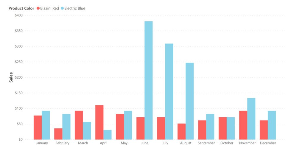
    We started this whole widget example with this premise: we have a hunch that blue widgets sell better in the summer, and we want to check our historical data to see if we’re right. Let’s up the stakes a bit- let’s imagine that we have the opportunity to go all-in on an expensive blue-widget marketing plan for June.

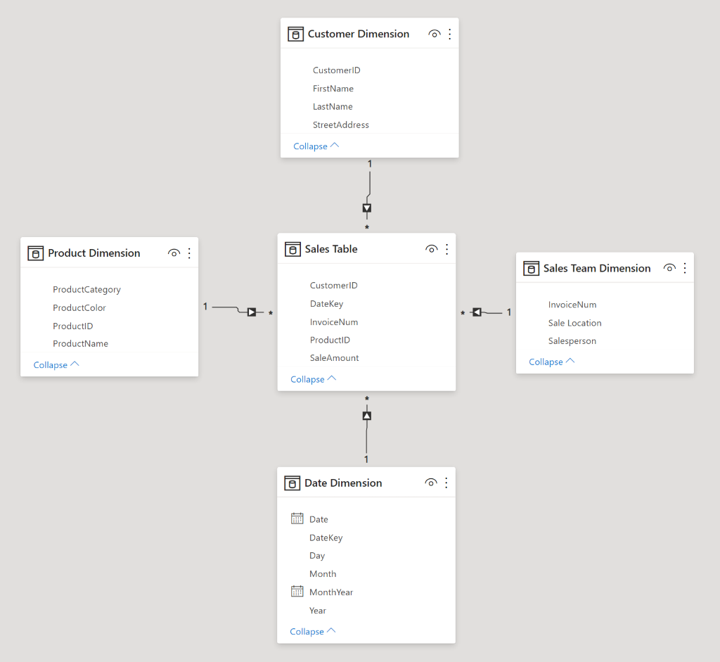
    On the advice of a friend, let’s say that we organized our widgety data into a star schema. Each sale is recorded in the fact table, and all the attributes that are related to each sale event (or ‘fact’) are organized into dimension tables. Then, we filtered our sales table by product, color, and month (we’ve accomplished this by creating relationships between tables in the model- something we’re about to dive into in this article).

    We see now the general monthly trends of widget sales, and checked our data, and blue widgets seem to be selling at a rate of 2 times that of red widgets in the summer. Aha!

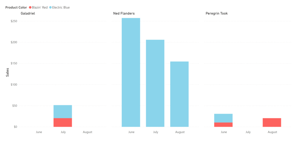
    It’s looking like it’s time to launch that Blue Widget Summer marketing campaign. We’re about to make the call and drop some real ca$h, when suddenly a breathless salesperson bursts into the room (it’s improbable, but go with me here). “Wait!” they say, “what about old Ed?” You scratch your head quizzically, but before you can chastise them for kicking the door down, they go on: “look at blue widget sales by customer”.

    So you do (which takes seconds thanks to your star schema), and lo and behold, it looks like 95% of your blue widgets sales were made to one person: Ned Flanders. Ned was 60 back in 1989 when the Simpsons first aired, which puts him at death’s door (or at least on death’s porch).

    Uh-oh. You were thinking you were going to capitalize on summer blue-widget fervor. But it turns out, Ned only leaves his house in the warmer months, and is a compulsive blue widgeteer. Good thing your salesperson has legs strong enough to kick down office doors. You make a mental note not to skip leg day at the gym.

    The power of a fully realized data model is being able to quickly investigate your data from multiple perspectives. Slicing sales by customer, by location, by date, or by product attributes is fast (‘slicing’ is a synonym for filtering data- it’ll be more clear why the verb slicing is used when we dig into data cubes). In our second article we mentioned that data models become more complex when our questions become more time sensitive. Star schemas help us answer questions quickly, taking advantage of relationships.

    What is a relationship?

    People have been trying to understand love for thousands of years, and lucky for me, that’s not the kind of relationship we’re talking about here. When I talk about relationships in this series, I’ll be talking about relationships in databases or data models.

    Relationships link two tables together, connecting a column in one table with a column in a second table.

    Table 1: A sample fact table
    Table 2: A sample (simplified) date dimension table
    Table 3: A sample customer dimension table
    Table 4: A sample product dimension table

    I’ve highlighted the relationships with blue, gold, and green above – Date with Date, Customer ID with Customer ID, and Product ID with Product ID. Column names need not match in the real world, I’ve made them match here for clarity. Take a moment and see what you can infer about the sales listed in Table 1. Who purchased what? Not every row in the fact table has visible matching rows in the dimension tables – they’re abridged in this example and would continue for many more rows.

    Sidebar: The Case of the Invisible Data, Again
    Notice how Table 2 above contains a date for which we had no sales. This is important – the date dimension is continuous, even if we don’t make sales every day. We’ll write more on that topic in the upcoming Case of the Invisible Data. For now know that sometimes it’s as important to know which days you had no sales as it is to know which days you had sales.

    Relationships allow you to filter data. Take for example a sum of sales. If I sum up my sales, I would get a single number: the combined amount of every sale ever.

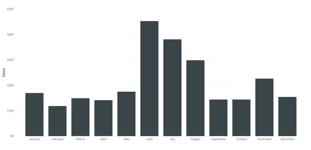
    Although that’s useful on days when we’re feeling down about life, there’s not a lot of nuance there with which to make decisions. What if we summed up our total sales, but used month as a dimension? We’d then see the sum of any sale made in any January next to any sale made in any February and on and on.

    That’s getting more useful (we could examine seasonal trends over many years). It might be helpful to add year in as well, so January 2018 is different from January 2019. To get these sums, we could go in and manually add up each sale in each month, or we could let the computer do that for us by creating a relationship.

    With a relationship, we can ask for the sum of sales, and filter by the Month Year column in the date dimension. Since we’ve established a relationship, the filter travels from the date dimension to the fact table. In order for the relationship to usefully accomplish this, for each instance of Date in the fact table, there must be only one corresponding row in the date dimension table. This is called a many-to-one relationship, because there are many instances of a given date in the fact table which correspond to one instance of that date in the dimension table.

    Furthermore, filters travel one direction along this relationship, making it a directional relationship. It’s useful to see all the sales made to one customer (many-to-one relationship, where the filter travels from the customer dimension to the sales fact table). It’s not as useful to see all the customers that were part of one sale (that’s typically one). Many data modelling programs (like Power BI) require many-to-one relationships by default, and similarly require the directionality be from the one side to the many side. The result is dimensions filtering the fact table. For instance, if we have 12 sales on January 1, 2019, that’s fine. If however January 1, 2019 shows up twice in the date dimension (and thus on the axis of the resulting visualization), we have a problem – where do January 1, 2019 sales go? There are bi-directional relationships and many-to-many relationships, but these complex relationships address very specific scenarios that we’ll be covering in a separate article.

    You can see many-to-one directional relationships in Figure 1 at the beginning of this article (a star schema created in Power BI). The many side is marked with an asterisk * and the one side is marked with a 1. The directionality is indicated with an arrow.

    Where are my keys?

    The kind of gobble-de-gook that gums up the process of learning business intelligence

    To rephrase something I wrote above: each row in a dimension table must be unique (in a typical many-to-one relationship). To be unique, there must be a column that contains a unique value in each row (the column has maximum cardinality). The column that uniquely identifies each row in a table is called a primary key. Each of the highlighted columns in the four tables above are keys. There are three kinds of keys I’ll be covering below, any of which can be used as a primary key.

    Natural Keys

    Natural keys already exist in your data. In the example above, Date is a natural key. To be stored as a number, the date can also be organized in the format YYYYMMDD (June 1, 2019 becomes 20190601). In the USA where I live, Social Security Number is a natural key. Each US citizen is assigned one at birth, and each number is (supposedly) unique. When building a date dimension, date can serve as the key – there’s no need to establish a code to represent each date.

    For the customer table, you might think that full name is a good candidate for a natural key. It isn’t because names aren’t consistent (and they’re not as unique as you might think). Take Galadriel for example. If the Lady of Lothlórien wanted to go by Altáriel (as she sometimes does) and we were using name as a natural key, we would need to update that record in dozens of places in our database: once in the customer dimension table, and then again for every row in the fact table where she was the customer. It’s much easier to keep her customer ID the same and update her name. Additionally, though she goes by many names, she doesn’t have a last name. She’s a rocker like Sting, or Bono, or Cher, or Madonna. The variabilities of names can create problems in our dataset.

    Surrogate Keys

    To handle the issue with customer name, we created a surrogate key. It’s an arbitrary number and has no bearing on the world outside of our data model. It started at 1 and incremented from there. Ned Flanders might take some joy from being customer #1, but him telling me that at a dinner party wouldn’t exactly impress me.

    Composite Keys

    Composite keys are similar to natural keys in that they’re made up of real-world attributes. The difference is that a composite key is, well, composite. By combining two or more columns that aren’t themselves unique, we end up with a unique column. In our example above, instead of creating a Product Number, we could have created a composite key out of ProductName and Product Color. The result would have been a column with values like Widget Classic Blazin’ Red, and Ball Cap Acid Green. One problem with composite keys is that as you add data, it’s possible you can end up with duplicates. Perhaps we add a new product category – Convention Widgets. We sell the same widgets in the standard colors at conventions, so they’re in a different product category. Our composite key would have two entries for Widget Classic Blazin’ Red, and that would be problematic.

    Other Keys

    As I wrote above, the column that uniquely identifies each row in a table is called a primary key. It doesn’t matter if it’s a natural key, a surrogate key, or a composite key. As long as it uniquely identifies the row, it’s the primary key. There a few more definitions that are worth knowing, especially as you do more work at the data prep level:

    A column which uniquely identifies each row in a table is also called a unique key. Primary keys are unique keys, and a single table can have many unique keys.

    Any column that could serve as a primary key is a candidate key, and the ones that aren’t chosen are alternate keys.

    Each of the primary keys in the dimension tables (Date, Customer ID, and Product ID) are called foreign keys in the fact table. They’re foreign keys in the fact table because they refer to the primary key of other tables.

    Sidebar: Fact Tables, Primary Keys, and Cardinality
    The fact table in our example above (Table 1) has its own primary key, Invoice Number (which happens to be a surrogate key). If, for whatever reason, your model doesn’t capture information at the grain of individual sales, or you’re only interested in summaries rather than being able to investigate specific sales, there’s nothing inherently wrong with omitting a Invoice Number or an arbitrary key from a fact table.

    Remember, each row in a fact table does not need to be unique. In fact, compression benefits from each row not being unique. They often are – if an invoice number or sales order number is included in a sales fact table, each row will end up being unique.  Software engines are smart enough to ignore keys when compressing the data; including a natural key or adding a surrogate key in a fact table doesn’t automatically put you at maximum cardinality.

    With that, it’s time to take a break. Literally stand up (if you aren’t standing from the joy of learning already), reach for the skies above, reach for your toes, wiggle your spine, and share what you’ve learned (perhaps with a notepad or animal companion). We have one more article (I promise it’s on the less technical side) in this introductory series, where we explore more deeply the ‘why’ of BI.


    Sign up to receive email notifications when we release new learning content

    Sources

    1. Data Modeling for Power BI – Online Course from https://www.sqlbi.com/
    2. https://www.databasestar.com/database-keys/